For my capstone project as a Flatiron Data Science student, I decided to take a crack at a Kaggle competition: LANL Earthquake Prediction. I chose this competition because I thought it would be a good way to stretch myself out of my confort zone, which turned out to be true! It was challenging in a number of ways:
- The datafile was larger than any I’ve worked with (over 600M rows of data)
- The data were raw signal data, which I have never worked with
- The modeling required that I develop a sophisticated cross-validation strategy to ensure success in the competition
As you’ll see in my write-up, I had moderate success addressing each of these challenges. At the end, I’ll discuss some things I would try in order to improve the modeling, given more time and computing power. I feel successful insofar as I was able to make some progress, and I got to learn how much more I have to learn. This project reminded me that there is always more work to be done, that perfection is an unattainable goal, and that, as the saying goes, “all models are wrong, but some are useful.”
Overview
The data for the competition were collected from earthquake simulations in a laboratory setting. The competition aims to solve the following problem: is it possible to predict the timing of aperiodic earthquakes using acoustic data recorded before the earthquake? Prior work showed that the prediction of laboratory earthquakes from continuous seismic data is possible in the case of quasi-periodic laboratory seismic cycles. However, aperiodic eqarthquakes remain difficult to predict.
Under the constraints of the competition rules, I find that it is possible to use tree-based regression algorithms to improve the prediction of laboratory earthquakes using features engineered from raw acoustic data. While these models yield a substantial improvement over a dummy model, they still include a substantial amount of error. Nonetheless, these models may still be useful for further seismology research and for future development of public earthquake early-warning systems.
Below, I provide an overview of the analysis using the OSEMN framework. You can see the full analysis at My Github Repository.
Obtaining the data
Since the raw data were so long, importing and working with the data was not trivial. Because the competition required that we make predictions based on acoustic snippets with 150,000 rows, I had to break the original 600M row training file into segments of that size. In this post, I go into detail about some of the challenges associated with importing and segmenting the data. I ultimately created about 13,000 snippets from the original datafile to use for my analysis.
Scrubbing the data
The next challenge was to process the 13,000 snippets to generate a set of features to use in my analysis. With limited knowledge of the topic, I had to do a fair amount of research on signal processing.
First, I explored functions that can be used to summarize signal data. I started with just using basic functions I knew, such as standard deviations and means. I then branched out into other summary functions, such as rolling averages and Hann windows. Lastly, I found a python package, tsfresh, that contained a number of functions for processing time series data. Using these functions with various parameter combinations, I came up with about 400 feature generating functions.
Next, I explored transformations of the original raw datafile that I might do before applying the summarizing functions. One transformation I used was wavelet denoising, which removes the “artificial impulse” introduced by the measurement device. Another transformation was the Fast Fourier Transform, which produces two additional transforms of the original data (real and imaginary). I used each combination of these transformations (raw vs denoised, no-FFT vs real FFT vs imaginary FFT), yielding 6 total transformations to use to generate features. Thus, I ended up with about 2,400 features.
Many of these features were either redundant or useless for classification. I dropped all features that had correlations with other features above 0.99, and I dropped any features with correlations below 0.005 with the target variable, time to failue. In the end, I retained 905 features to use in my analyses.
Exploring the data
Here is one viaulization that gives an overview of the training dataset:
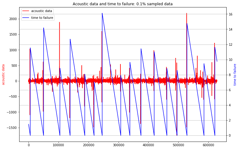
The red line is the raw acoustic data, which you can see oscillates somewhat over the course of the full training set. There are a few large oscillations that occur periodically throughout. Some of these large oscillations occur when an earthquake happens, but some do not.
The blue line shows the target variable, “time to failure”, which captures the time until an earthquake occurs. Time to failure decreases over time during the intervals between earthquakes. The large vertical jumps in the blue line show the times when an earthquake happened. When an earthquake occurs, the time to failure is 0, and then jumps up to a value representing the time until the next earthquake.
Modeling the Data
I used to approaches to modeling the data: random forests and gradient boosting machines. I chose to use tree-based methods because they are good at handling problems with large numbers of features. Gradient boosting machines turned out to be much faster without much loss of performance. I removed some features during the modeling stage after seeing that they had low feature importance. I then used cross validation to tune hyperparameters for these models.
Cross-validation was a difficult challenge for this problem. I created a holdout set with 20% of the data to use for testing my models. Hoever, because many of the samples contained overlapping acoustic data, I had to ensure that the holdout set did not include raw data that would be present in the training set. It was not possible to do this perfectly, so I reduced the amount of overlap by removing a sample of acoustic snippets that overlapped as much as possible. I used this holdout set to test the performance of models after hyperparameter tuning.
Interpreting the models
Her are the results:

Both the random forest and gradient-boosting machine trees give comparable performance, both in terms of their cross-validation metrics and performance on Kaggle’s evaluation set. They are generally able to predict time to failure with an average error of about 2 seconds. While this is a substantial improvement of the dummy regressor, which had an error of 3 seconds, it is still a fairly large amount of error. Interestingly, the performance is better on Kaggle than for the cross-validation, presumably because the sample of snippets being used for evaluation have fewer extreme values.
The lack of any clear cutoffs for feature importances also gives me reason for concern. There were a couple stand-out features from the random forest model, but for the most part, most features seem to add little information. While I was able to remove a large number of less useful ones, I don’t have confidence that I have created many features that indivudally capture much of the important variation in time to failure. It is possible that this problem requires a new approach to signal processing to generate better features.
Conclusion
There a number of next steps to pursue to improve the performance of this model:
- Conduct more research on signal processing to better generate features that are likely to be useful for this problem
- Better reduce feature space by using PCA and tuning the feature importance cutoff
- Conduct more extensive hyperparameter tuning
- Develop a more robust cross-validation strategy
- Use new models, such as a neural network on top of calculated features or a 1D CNN
Even with these additional steps, I still believe that the structure of this problem is such that it will be difficult to generate a robust model. This is because the training data only includes 16 failures, which means that there is limited information about time to failure in the dataset. Each period before a failure is quite distinct, so additional data would improve the training in the model. In addition, the challenge of predicting time to failure on a short snippet of acoustic data is much harder than trying to predict failures with more longitudinal data. Lastly, lack of information about the time that samples were collected in the test set prevent analyses of acoustic data at different time scales in a fine-grained way. Thus, additional data are needed to produce a robust solution to this problem.